BVPelectrostatic2D01

% -----------------------------------------------------
% Solving a BVP by using <fc-vfemp1>
% -----------------------------------------------------
% 2D condenser BVP[01] on GMSH mesh from
%         square4holes6dom.geo,
%    mesh of the on square [-1,1]x[-1,1]
%    with 4 holes and 6 domains
% -----------------------------------------------------
%  PDE :
%    * -div(sigma grad(phi)) = 0   on domain [2,4,6,8,10,20]
%  Local electrical conductivity :
%    * sigma=sigma1=1  on domain [10]
%    * sigma=sigma2=10 on domain [2,4,6,8,20]
%  Dirichlet boundary condition on boundaries [1,3,5,7]
%    * on [1,5] : phi = 12
%    * on [3,7] : phi = 0
%  Neumann boundary condition on boundary [20]
%    * on [20] : sigma d(phi)/dn = 0
% -----------------------------------------------------
close all
clear all
geofile='square4holes6dom.geo';
fullgeofile=fc_vfemp1.get_geo(2,2,geofile);
if isempty(fullgeofile), error('geofile %s not found',geofile);end
% Building the mesh using GMSH
meshfile=fc_oogmsh.gmsh.buildmesh2d(fullgeofile,30);
% Loading the mesh using <fc_simesh.siMesh> object
Th=fc_simesh.siMesh(meshfile);
Th.info('verbose',true)
%
% SETTING THE BVP
%
sigma1=1;sigma2=10;
% Setting -Laplacian operator
Lop1=fc_vfemp1.Loperator(2,2,{sigma1,0;0,sigma1},[],[],[]);
Lop2=fc_vfemp1.Loperator(2,2,{sigma2,0;0,sigma2},[],[],[]);
% Setting the PDE : -Laplacian(u) = 0
pde1=fc_vfemp1.PDE(Lop1);
pde2=fc_vfemp1.PDE(Lop2);
% Setting the BVP
bvp=fc_vfemp1.BVP(Th,pde2); % set pde2 to all the domains [2,4,6,8,10,20]
bvp.setPDE(2,10,pde1);      % set pde1 to domain [10]
bvp.setDirichlet( 1, 12);
bvp.setDirichlet( 3, 0);
bvp.setDirichlet( 5, 12);
bvp.setDirichlet( 7, 0);
% Default boundary condition is Homegeneous Neumann:

%
% SOLVING THE BVP
%
fprintf('*** Solving the potential phi\n')
phi=bvp.solve();

%
% COMPUTING THE ELECTRIC FIELD E=-grad phi
%
fprintf('*** Computing the electric field E\n')
Lop=fc_vfemp1.Loperator(2,2,[],[],{-1,0},[]);
Ex=Lop.apply(Th,phi); % Ex= - d phi/ dx
Lop=fc_vfemp1.Loperator(2,2,[],[],{0,-1},[]);
Ey=Lop.apply(Th,phi); % Ey= - d phi/ dy
E=[Ex,Ey];
ENorm=sqrt(Ex.^2+Ey.^2);

%
% GRAPHICS
%
fc_tools.graphics.monitors.onGrid(3,3,'figures',1:7,'covers',0.9);
interpreter=@(x) fc_tools.graphics.interpreter(x);
if fc_tools.comp.isOctave(),opt_interp={'interpreter','tex'};else,opt_interp={'interpreter','latex'};end

tstart=tic();
figure(1)
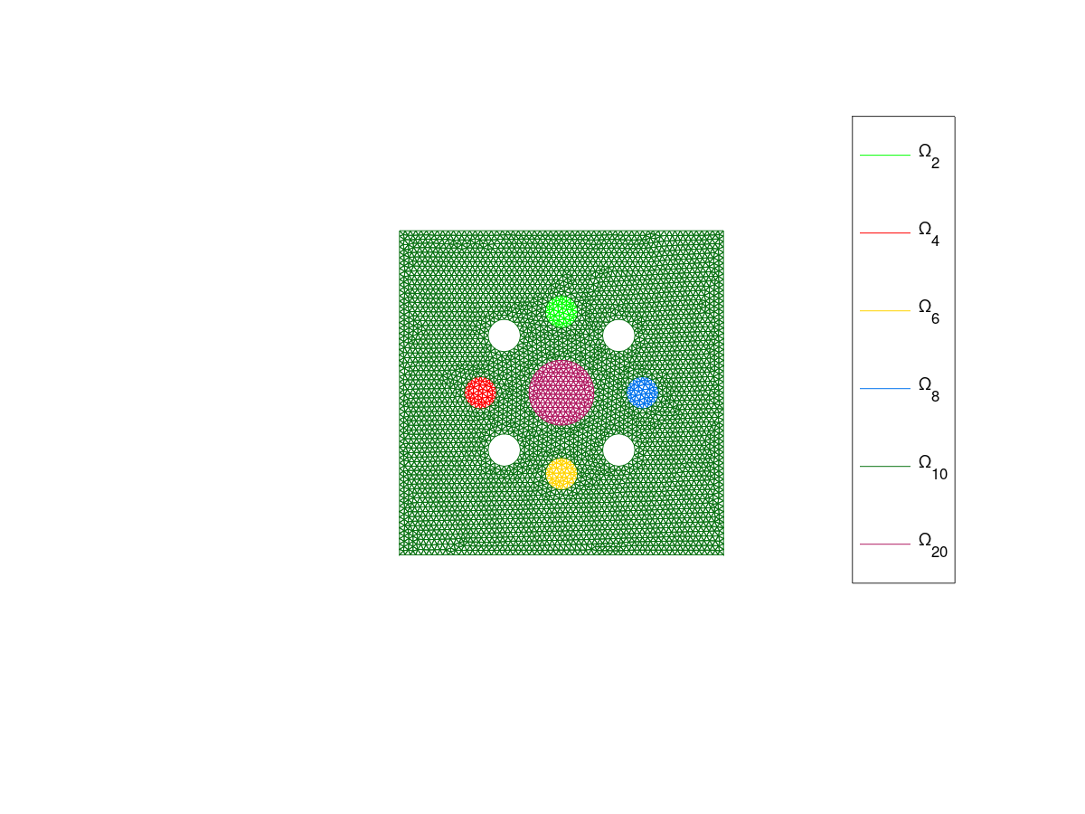
Th.plotmesh('inlegend',true)
legend('show')
axis equal;axis off

figure(2)
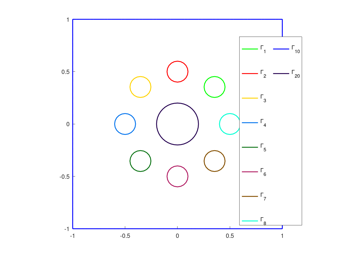
Th.plotmesh('color',[0.8,0.8,0.8])
Th.plotmesh('d',1,'LineWidth',1.5,'inlegend',true)
legend('show')
axis image

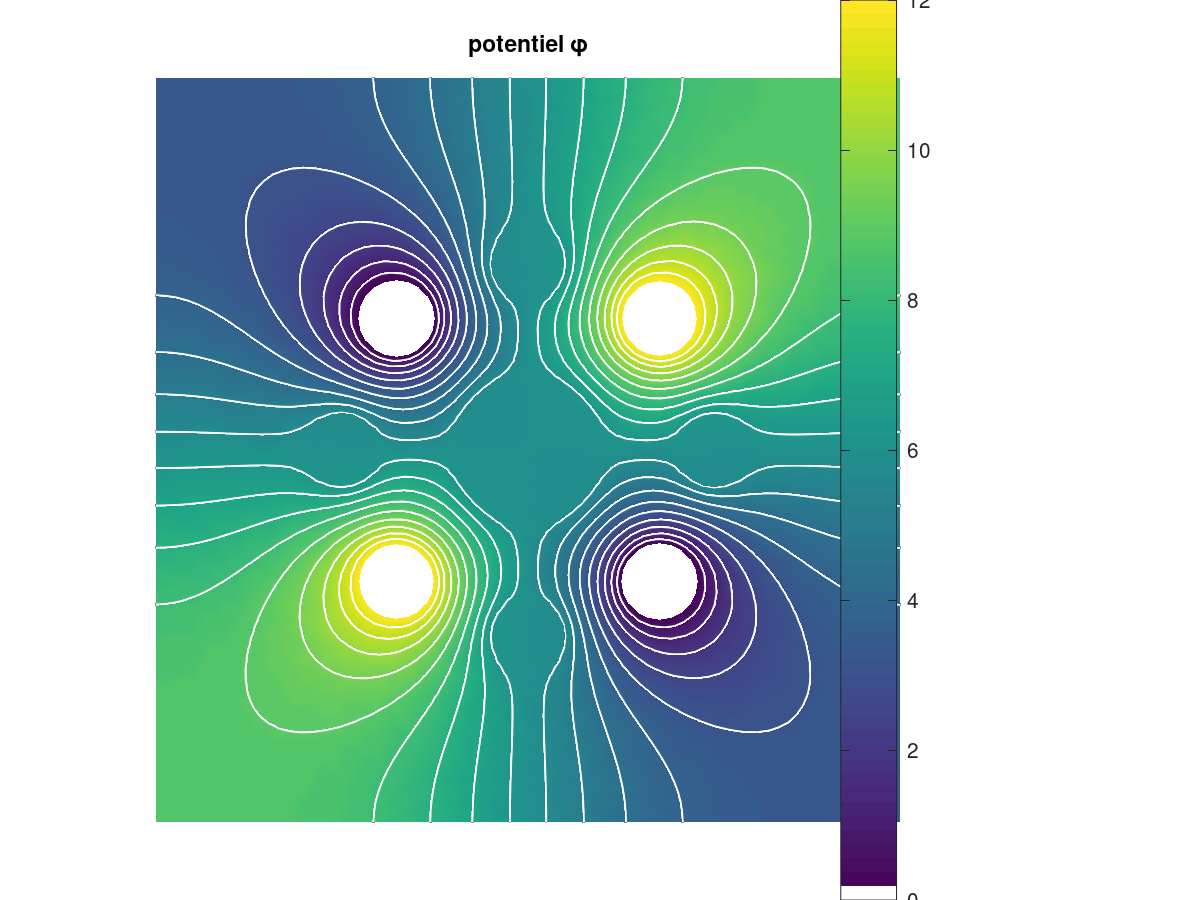
figure(3)
Th.plotmesh('d',1,'color',[0,0,0])
hold on
Th.plot(phi,'EdgeColor','None')
axis image;axis off;
colorbar()
Th.plotiso(phi,'niso',20,'color','w','LineWidth',1)
Th.plotmesh('d',1,'color','w','LineWidth',1.5)
shading interp
title(interpreter('potentiel $\varphi$'),opt_interp{:})

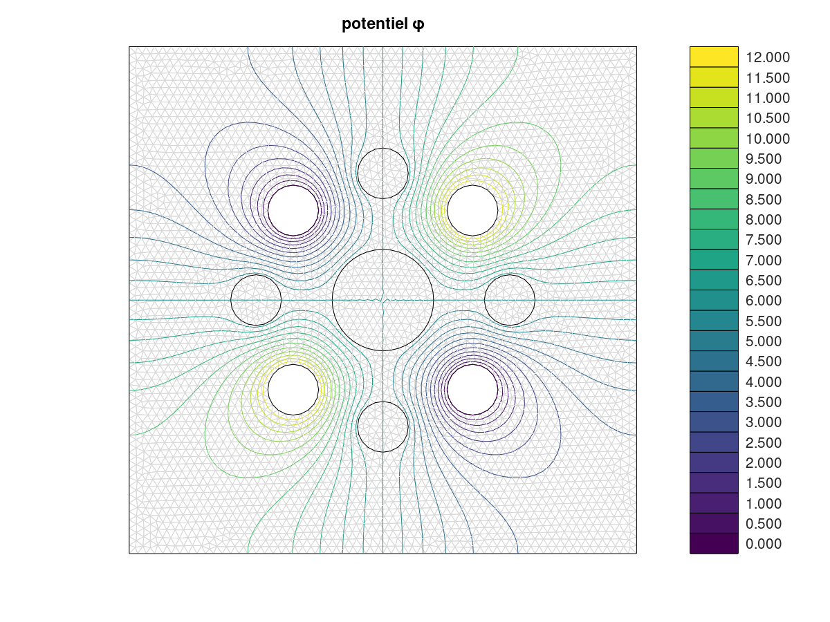
figure(4)
Th.plotmesh('color',[0.85,0.85,0.85])
hold on
Th.plotmesh('d',1,'color',[0,0,0])
[~,~,cax]=Th.plotiso(phi,'niso',25,'isocolorbar',true,'format','%.3f');
axis image;axis off;
title(interpreter('potentiel $\varphi$'),opt_interp{:})

idxlab=Th.find(2,10);
figure(5)
Th.plotmesh('d',1,'color','k')
hold on
[~,~,cax]=Th.plotiso(phi,'niso',25,'isocolorbar',true,'format','%.3f');
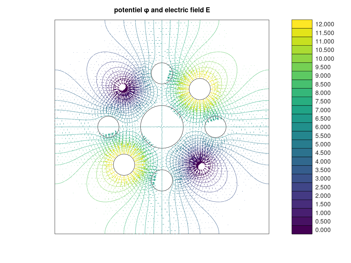
Th.plotquiver(E,'d',2,'labels',[10],'colordata',phi)
axis image;axis off;
title(interpreter('potentiel $\varphi$ and electric field $E$'),opt_interp{:})

figure(6)
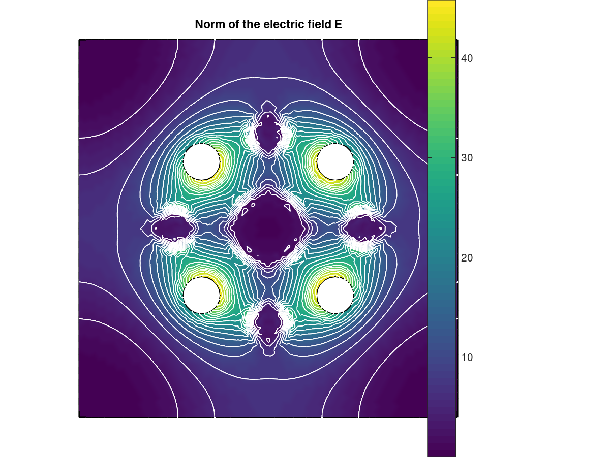
Th.plot(ENorm,'EdgeColor','None')
hold on
axis image;axis off;
colorbar()
Th.plotiso(ENorm,'niso',20,'color','w','LineWidth',1)
Th.plotmesh('d',1,'color','k','LineWidth',1.5)
shading interp
title(interpreter('Norm of the electric field $E$'),opt_interp{:})

figure(7)
Th.plotmesh('d',1,'color',[0,0,0])
hold on
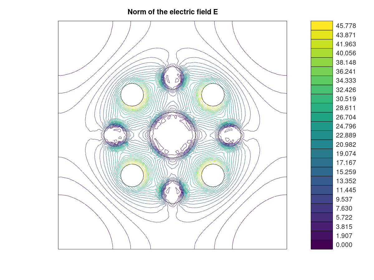
[~,~,cax]=Th.plotiso(ENorm,'niso',25,'isocolorbar',true,'format','%.3f');
axis image;axis off;
title(interpreter('Norm of the electric field $E$'),opt_interp{:})

[fc-oogmsh] Input file : /home/cuvelier/Travail/Recherch/Matlab/fc-vfemp1/geodir/2d/square4holes6dom.geo
[fc-oogmsh] Mesh file <fc-oogmsh>/meshes/square4holes6dom-30.msh [version 4.1] already exists.
  -> Use "force" flag to rebuild if needed.
Variable  [fc_simesh.siMesh object] :
  dim=2, d=2
  nq=4632, nme=8950
  2-simplices : number 6, labels : 2 4 6 8 10 20 
  1-simplices : number 10, labels : 1 2 3 4 5 6 7 8 10 20 
  0-simplices : none
*** Solving the potential phi
*** Computing the electric field E