Element Mass Matrix
We have
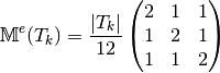
Then with  definition (see Section New Optimized assembly algorithm (OptV2 version)) , we obtain
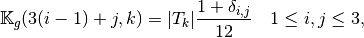
We represent in figure 13 the corresponding row-wise operations.
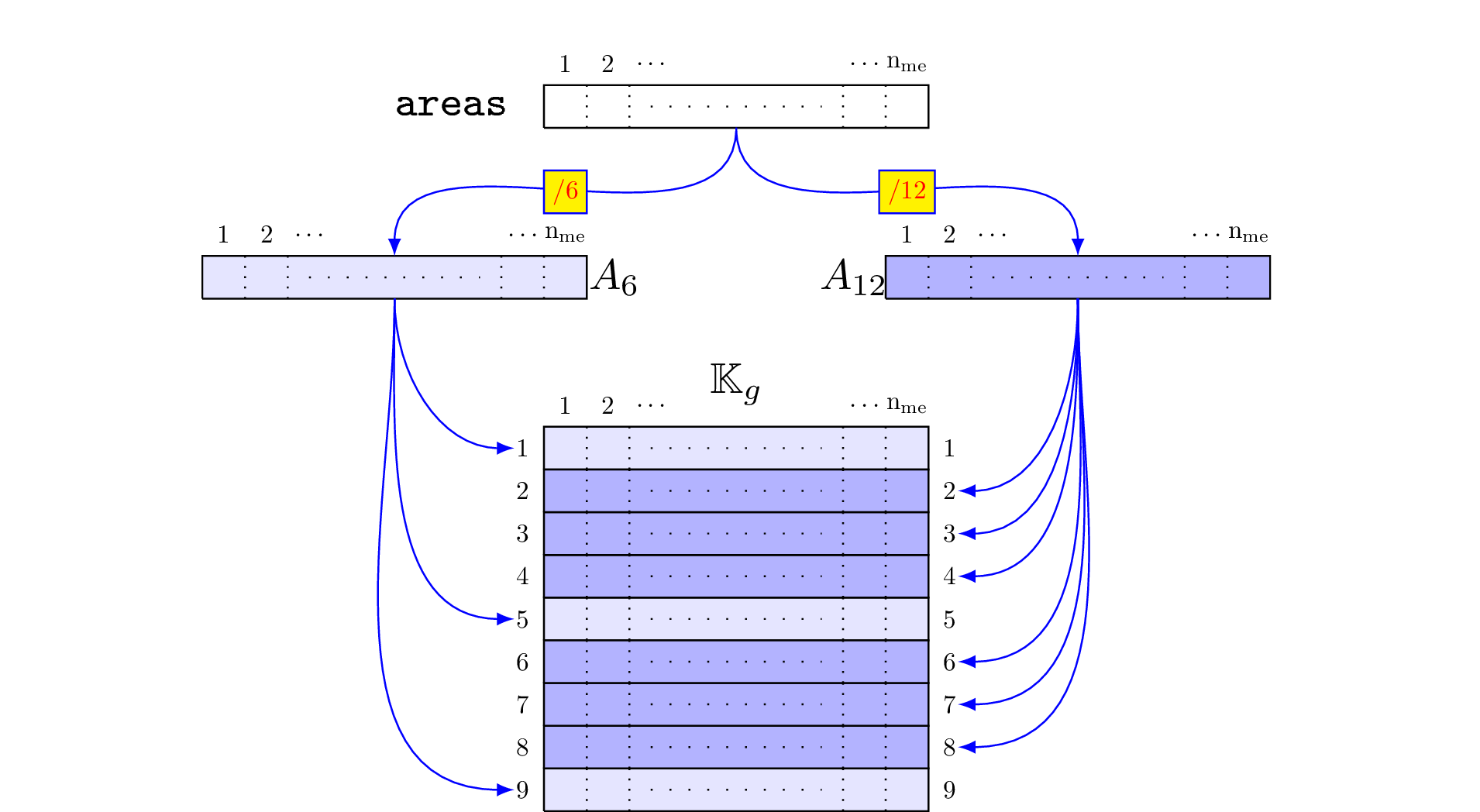
Figure 13: Construction of  associated to 2d Mass matrix in
So the vectorized algorithm for computation is simple and given in Algorithm 14.
Algorithm 14
Figure 14: Vectorized algorithm for associated to 2d Mass matrix
Note
- pyOptFEM.FEM2D.elemMatrixVec.ElemMassMat2DP1Vec(areas)[source]
Computes all the element Mass matrices
 for
for 
Parameters: areas (  numpy array of floats) – areas of all the mesh elements.
Returns: a one dimensional numpy array of size 
Element Stiffness Matrix
We have 
Using vectorized algorithm function  given in Algorithm 12, we obtain
the vectorized algorithm 15 for computation for the Stiffness matrix in 2d.
given in Algorithm 12, we obtain
the vectorized algorithm 15 for computation for the Stiffness matrix in 2d.
Algorithm 15
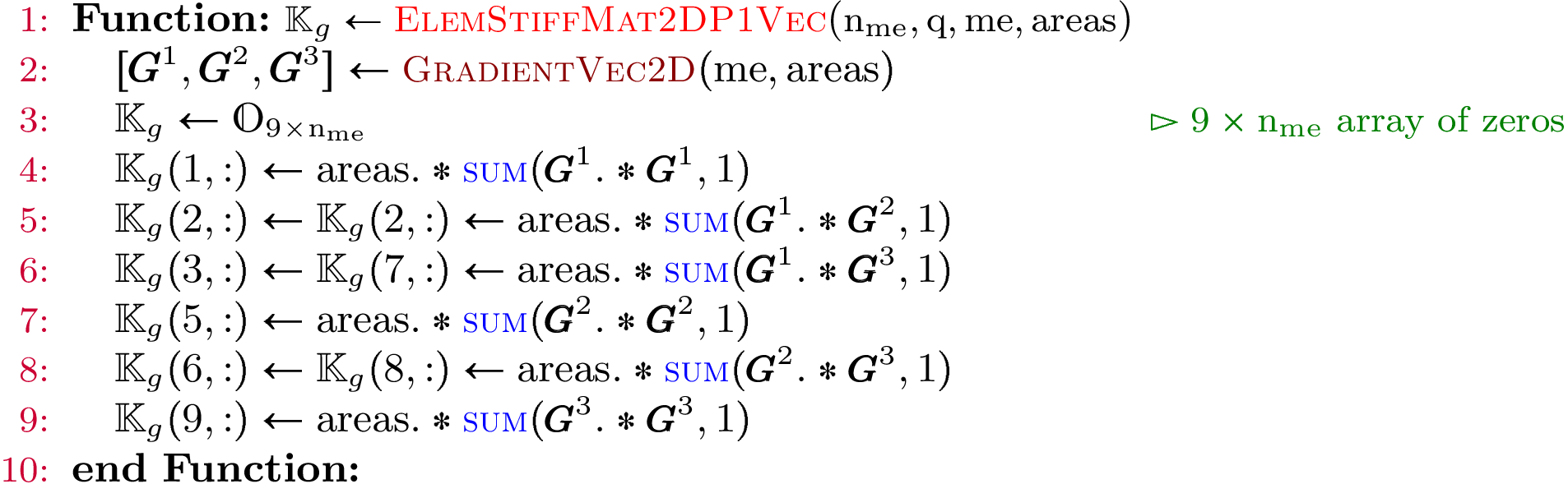
Figure 15: Vectorized algorithm for associated to 2d Stiffness matrix
Note
- pyOptFEM.FEM2D.elemMatrixVec.ElemStiffMat2DP1Vec(nme, q, me, areas)[source]
Computes all the element stiffness matrices
 for
for Parameters: - nme (int) – number of mesh elements,
- q (
 numpy array of floats) – mesh vertices,
 - me (
 numpy array of integers) – mesh connectivity,
 - areas ( numpy array of floats) – areas of all the mesh elements.
Returns: a one dimensional numpy array of size
Element Elastic Stiffness Matrix
We define on
 the local alternate basis
  by
by
where
 With notations of Presentation, we have
with,
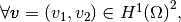
(1)
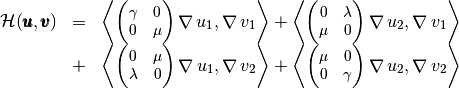
For example, we can explicitly compute the first two terms in the first column of
 which are given by
and
Using vectorized algorithm function
given in Algorithm 12, we obtain
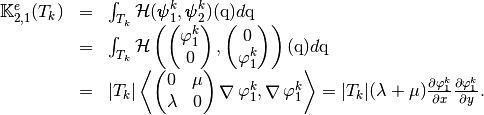
the vectorized algorithm 15 for computation for the Elastic Stiffness matrix in 2d.Algorithm 16
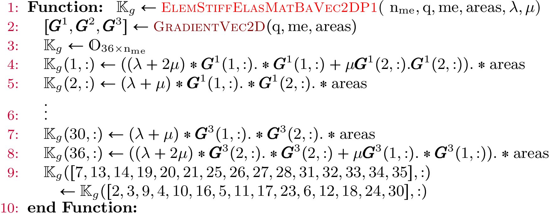
Figure 16: Vectorized algorithm for
associated to 2d Elastic Stiffness matrixNote
- pyOptFEM.FEM2D.elemMatrixVec.ElemStiffElasMatBaVec2DP1(nme, q, me, areas, L, M, **kwargs)[source]
Computes all the element elastic stiffness matrices
 for in local alternate basis.
Parameters: Returns: a (36*nme,) numpy array of floats.
We define on
the local block basis  by
by
where
For example, using formula (1), we can explicitly compute the first two terms in the first column of
which are given by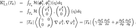
and

Using vectorized algorithm function
given in Algorithm 12, we obtain
the vectorized algorithm 17 for computation for the Elastic Stiffness matrix in 2d.Algorithm 17
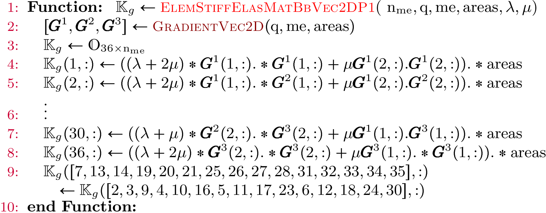
Figure 17: Vectorized algorithm for
associated to 2d Elastic Stiffness matrixNote
- pyOptFEM.FEM2D.elemMatrixVec.ElemStiffElasMatBbVec2DP1(nme, q, me, areas, L, M, **kwargs)[source]
Computes all the element elastic stiffness matrices
for in local block basis.Parameters: Returns: a (36*nme,) numpy array of floats.
 Lame parameter,
 Lame parameter.