FEM2D module
| Author: | Francois Cuvelier <cuvelier@math.univ-paris13.fr> |
|---|---|
| Date: | 15/09/2013 |
Contains functions to build some finite element matrices using  -Lagrange finite elements on a 2D mesh.
Each assembly matrix is computed by three differents versions called base,
OptV1 and OptV2 (see here)
-Lagrange finite elements on a 2D mesh.
Each assembly matrix is computed by three differents versions called base,
OptV1 and OptV2 (see here)
Contents
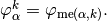
Assembly matrices (versions base, OptV1 and OptV2)
Let  be a triangular mesh of
  We note
  a triangulation of
  with the following structure data:
![\mbox{\begin{tabular}{lccll}
\hline
\textbf{name} & \textbf{type} & \textbf{dimension} & \textbf{description}& \textbf{Python}\\
\hline
$\nq$ & integer & 1 & number of vertices& \texttt{nq}\\
$\nme$ & integer & 1 & number of elements& \texttt{nme}\\
$\q$ & double & $2 \times \nq$ &
\begin{minipage}[t]{7.9cm}
array of vertices coordinates. $\q(\nu,j)$ is the $\nu$-th coordinate of the $j$-th vertex,
$\nu\in\{1,2\}$, $j\in\{1,\hdots,\rm{n_q}\}.$
The $j$-th vertex will be also denoted by $\rm{q}^j$
\end{minipage}&
\begin{minipage}[t]{3cm}
\texttt{q} (transposed)\\
\texttt{q[j-1]} = $\q^j$
\end{minipage}\\
$\me$ & integer & $3 \times \nme$ &
\begin{minipage}[t]{7.9cm}
connectivity array. $\me(\beta,k)$ is the storage index of the $\beta$-th vertex
of the $k$-th element, in the array~$q$, for $\beta\in\{1,2,3\}$ and $k\in\{1,\hdots,{\nme}\}$
\end{minipage}&\texttt{me} (transposed)\\
$\rm areas$ & double & $1\times {\nme}$ &
\begin{minipage}[t]{7.9cm}
array of areas. ${\rm areas}(k)$ is the $k$-th triangle area,
$k\in\{1,\hdots,{\nme}\}$
\end{minipage}&\texttt{areas}\\
\hline
\end{tabular}}](_images/math/11700f93ddb0ff30873e9fdaccf82333c1401a49.png)
The -Lagrange basis functions associated with  are noted
  for all
 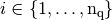 and are defined by

We also define the global alternate basis  by
by

and the global block basis  by
by

Mass Matrix
Assembly of the Mass Matrix by -Lagrange finite elements
using respectively version base, OptV1 and OptV2 (see report).
The Mass Matrix  is given by
Note
generic syntax:
M = MassAssembling2DP1<version>(nq,nme,me,areas)
- nq: total number of nodes of the mesh, also denoted by
 ,
, - nme: total number of triangles, also denoted by
 ,
, - me: Connectivity array, (nme,3) array,
- areas: Array of areas, (nme,) array,
- return a Scipy CSC sparse matrix of size

where <version> is base, OptV1 or OptV2
Benchmarks of theses functions are presented in Mass Matrix. We give a simple usage :
>>> from pyOptFEM.FEM2D import *
>>> Th=SquareMesh(5)
>>> Mbase =  MassAssembling2DP1base(Th.nq,Th.nme,Th.me,Th.areas)
>>> MOptV1= MassAssembling2DP1OptV1(Th.nq,Th.nme,Th.me,Th.areas)
>>> print(" NormInf(Mbase-MOptV1)=%e " % NormInf(Mbase-MOptV1))
NormInf(Mbase-MOptV1)=6.938894e-18
>>> MOptV2= MassAssembling2DP1OptV2(Th.nq,Th.nme,Th.me,Th.areas)
>>> print(" NormInf(Mbase-MOptV2)=%e " % NormInf(Mbase-MOptV2))
NormInf(Mbase-MOptV2)=6.938894e-18
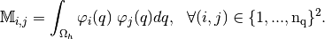
We can show sparsity of the Mass matrix :
>>> from pyOptFEM.FEM2D import *
>>> Th=SquareMesh(20)
>>> M=MassAssembling2DP1base(Th.nq,Th.nme,Th.me,Th.areas)
>>> showSparsity(M)
Figure 123: Sparsity of Mass Matrix generated with command showSparsity(M)
Note
sources code
- pyOptFEM.FEM2D.assembly.MassAssembling2DP1base(nq, nme, me, areas)[source]
Assembly of the Mass Matrix by
-Lagrange finite elements using base version (see report).
- pyOptFEM.FEM2D.assembly.MassAssembling2DP1OptV1(nq, nme, me, areas)[source]
Assembly of the Mass Matrix by
-Lagrange finite elements using OptV1 version (see report).
- pyOptFEM.FEM2D.assembly.MassAssembling2DP1OptV2(nq, nme, me, areas)[source]
Assembly of the Mass Matrix by
-Lagrange finite elements using OptV2 version (see report).
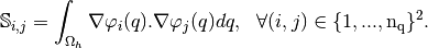
Stiffness Matrix
Assembly of the Stiffness Matrix by -Lagrange finite elements using respectively version base,
OptV1 and OptV2 (see report).
The Stiff Matrix  is given by
Note
generic syntax:
M = StiffAssembling2DP1<version>(nq,nme,q,me,areas)
- nq: total number of nodes of the mesh, also denoted by ,
- nme: total number of triangles, also denoted by ,
- q: Array of vertices coordinates, (nq,2) array
- me: Connectivity array, (nme,3) array,
- areas: Array of areas, (nme,) array,
- return a Scipy CSC sparse matrix of size
where <version> is base, OptV1 or OptV2
Benchmarks of theses functions are presented in Stiffness Matrix. We give a simple usage :
>>> pyOptFEM.FEM2D import *
>>> Th=SquareMesh(5)
>>> Sbase =  StiffAssembling2DP1base(Th.nq,Th.nme,Th.q,Th.me,Th.areas)
>>> SOptV1= StiffAssembling2DP1OptV1(Th.nq,Th.nme,Th.q,Th.me,Th.areas)
>>> print(" NormInf(Sbase-SOptV1)=%e " % NormInf(Sbase-SOptV1))
NormInf(Sbase-SOptV1)=0.000000e+00
>>> SOptV2= StiffAssembling2DP1OptV2(Th.nq,Th.nme,Th.q,Th.me,Th.areas)
>>> print(" NormInf(Sbase-SOptV2)=%e " % NormInf(Sbase-SOptV2))
NormInf(Sbase-SOptV1)=4.440892e-16
Note
sources code
- pyOptFEM.FEM2D.assembly.StiffAssembling2DP1base(nq, nme, q, me, areas)[source]
Assembly of the Stiff Matrix by
-Lagrange finite elements using base version (see report).
- pyOptFEM.FEM2D.assembly.StiffAssembling2DP1OptV1(nq, nme, q, me, areas)[source]
Assembly of the Stiff Matrix by
-Lagrange finite elements using OptV1 version (see report).
- pyOptFEM.FEM2D.assembly.StiffAssembling2DP1OptV2(nq, nme, q, me, areas)[source]
Assembly of the Stiff Matrix by
-Lagrange finite elements using OptV2 version (see report).
Stiffness Elasticity Matrix
Assembly of the Stiffness Elasticity Matrix by -Lagrange finite elements using respectively version base,
OptV1 and OptV2 (see report).
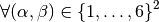
The Stiffness Elasticity Matrix  is given by
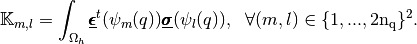
where
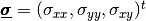 and
and
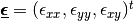 are the elastic stress and strain tensors respectively.
Note
generic syntax:
M = StiffElasAssembling2DP1<version>(nq,nme,q,me,areas,la,mu,Num)
nq: total number of nodes of the mesh, also denoted by
,nme: total number of triangles, also denoted by
,- q: array of vertices coordinates,
- (nq,2) array for base and OptV1,
- (2,nq) array for OptV2 version,
- me: Connectivity array,
- (nme,3) array for base and OptV1,
- (3,nme) array for OptV2 version,
areas: (nme,) array of areas,
la: the first Lame coefficient in Hooke’s law, denoted by
 ,
,mu: the second Lame coefficient in Hooke’s law, denoted by
 ,
,- Num:
- 0: global alternate numbering with local alternate numbering (classical method),
- 1: global block numbering with local alternate numbering,
- 2: global alternate numbering with local block numbering,
- 3: global block numbering with local block numbering.
return a Scipy CSC sparse matrix of size

where <version> is base, OptV1 or OptV2
Benchmarks of theses functions are presented in Stiffness Elasticity Matrix. We give a simple usage :
>>> from pyOptFEM.FEM2D import *
>>> Th=SquareMesh(5)
>>> Kbase =  StiffElasAssembling2DP1base(Th.nq,Th.nme,Th.q,Th.me,Th.areas,2,0.5,0)
>>> KOptV1= StiffElasAssembling2DP1OptV1(Th.nq,Th.nme,Th.q,Th.me,Th.areas,2,0.5,0)
>>> print(" NormInf(Kbase-KOptV1)=%e " % NormInf(Kbase-KOptV1))
NormInf(Kbase-KOptV1)=8.881784e-16
>>> KOptV2= StiffElasAssembling2DP1OptV2(Th.nq,Th.nme,Th.q,Th.me,Th.areas,2,0.5,0)
>>> print(" NormInf(Kbase-KOptV2)=%e " % NormInf(Kbase-KOptV2))
NormInf(Kbase-KOptV2)=1.776357e-15
We now illustrate the consequences of the choice of the global basis on matrix sparsity
global alternate basis
(Num=0 or Num=2)>>> from pyOptFEM.FEM2D import * >>> Th=SquareMesh(15) >>> K0=StiffElasAssembling2DP1OptV1(Th.nq,Th.nme,Th.q,Th.me,Th.areas,2,0.5,0) >>> showSparsity(K0)

Figure 124: Sparsity of Stiffness Elasticity Matrix generated with global alternate numbering (Num=0 or 2)
>>> K3=StiffElasAssembling2DP1OptV1(Th.nq,Th.nme,Th.q,Th.me,Th.areas,2,0.5,3)
>>> showSparsity(K3)
global block basis
(Num=1 or Num=3)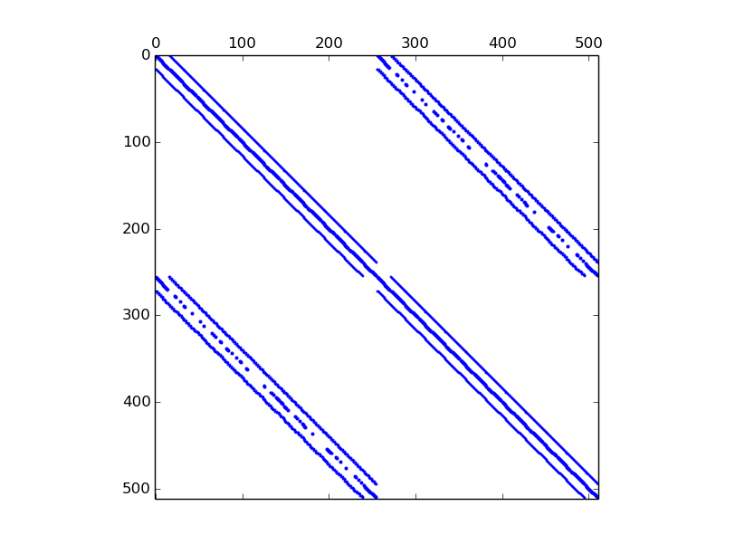
Figure 125: Sparsity of Stiffness Elasticity Matrix generated with global block numbering (Num=1 or 3)
Note
sources code
- pyOptFEM.FEM2D.assembly.StiffElasAssembling2DP1base(nq, nme, q, me, areas, la, mu, Num)[source]
Assembly of the Stiffness Elasticity Matrix by
-Lagrange finite elements using OptV2 version (see report).
- pyOptFEM.FEM2D.assembly.StiffElasAssembling2DP1OptV1(nq, nme, q, me, areas, la, mu, Num)[source]
Assembly of the Stiffness Elasticity Matrix by
-Lagrange finite elements using OptV1 version (see report).
- pyOptFEM.FEM2D.assembly.StiffElasAssembling2DP1OptV2(nq, nme, q, me, areas, la, mu, Num)[source]
Assembly of the Stiffness Elasticity Matrix by
-Lagrange finite elements using OptV2 version (see report).
Elementary matrices (used by versions base and OptV1)
Let  be a triangle, of area
  and with
  ,
,  and
and  its three vertices. We denote by
 ,
,  and
and  the -Lagrange local basis functions such that
  .
.
We also define the local alternate basis  by
by

and the local block basis  by
by

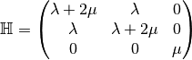
The elasticity tensor,  , obtained from Hooke’s law with an isotropic material,
defined with the Lamé parameters and is given by
, obtained from Hooke’s law with an isotropic material,
defined with the Lamé parameters and is given by
and, for a function  the strain tensors is given by
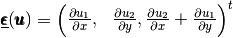
 , for the triangle
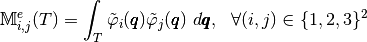
Element Stiffness Matrix
The element Stiffness matrix,  ,
for the is defined by
,
for the is defined by

We have :
where  ,
,  and
and  .
.
 numpy array) – the three vertices of the triangle,
Element Stiffness Elasticity Matrix
Let , and .
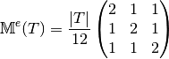
The element Stiffness Elasticity matrix,
 ,
for a given triangle in the local alternate basis is defined by
,
for a given triangle in the local alternate basis is defined by
We also have
where
is the elasticity tensor and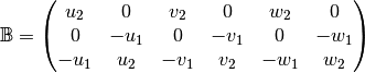
Note
- pyOptFEM.FEM2D.elemMatrix.ElemStiffElasMat2DP1Ba(ql, area, H)[source]
Return the element Stiffness Elasticity matrix,
,
for a given triangle in the local alternate basis Parameters: - ql (
 numpy array) – contains the three vertices of the triangle : ql[0], ql[1] and ql[2],
 - area (float) – area of the triangle ,
- H (
 numpy array) – Elasticity tensor, .
Returns: in basis.Type :  numpy array of floats.
- ql (
The element Stiffness Elasticity matrix,
,
for a given triangle in the local block basis is defined by
We also have
where
is the elasticity tensor and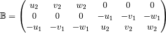
Note
- pyOptFEM.FEM2D.elemMatrix.ElemStiffElasMat2DP1Bb(ql, area, H)[source]
Return the element Stiffness Elasticity matrix,
,
for a given triangle in the local block basis Parameters: - ql ( numpy array) – contains the three vertices of the triangle : ql[0], ql[1] and ql[2],
- area (float) – area of the triangle,
- H ( numpy array) – Elasticity tensor, .
Returns: in basis.Type : numpy array of floats- ql (
Vectorized tools (used by version OptV2)
Vectorized computation of basis functions gradients
By construction, the gradients of basis functions are constants on each element  So, we denote,
 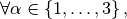 by
by  the
the  array defined,
 by
by

On a triangle  we denote by
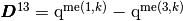 and
and
 Then, we have

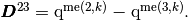
With these formulas, we obtain the vectorized algorithm given in Algorithm 134.
Algorithm 134
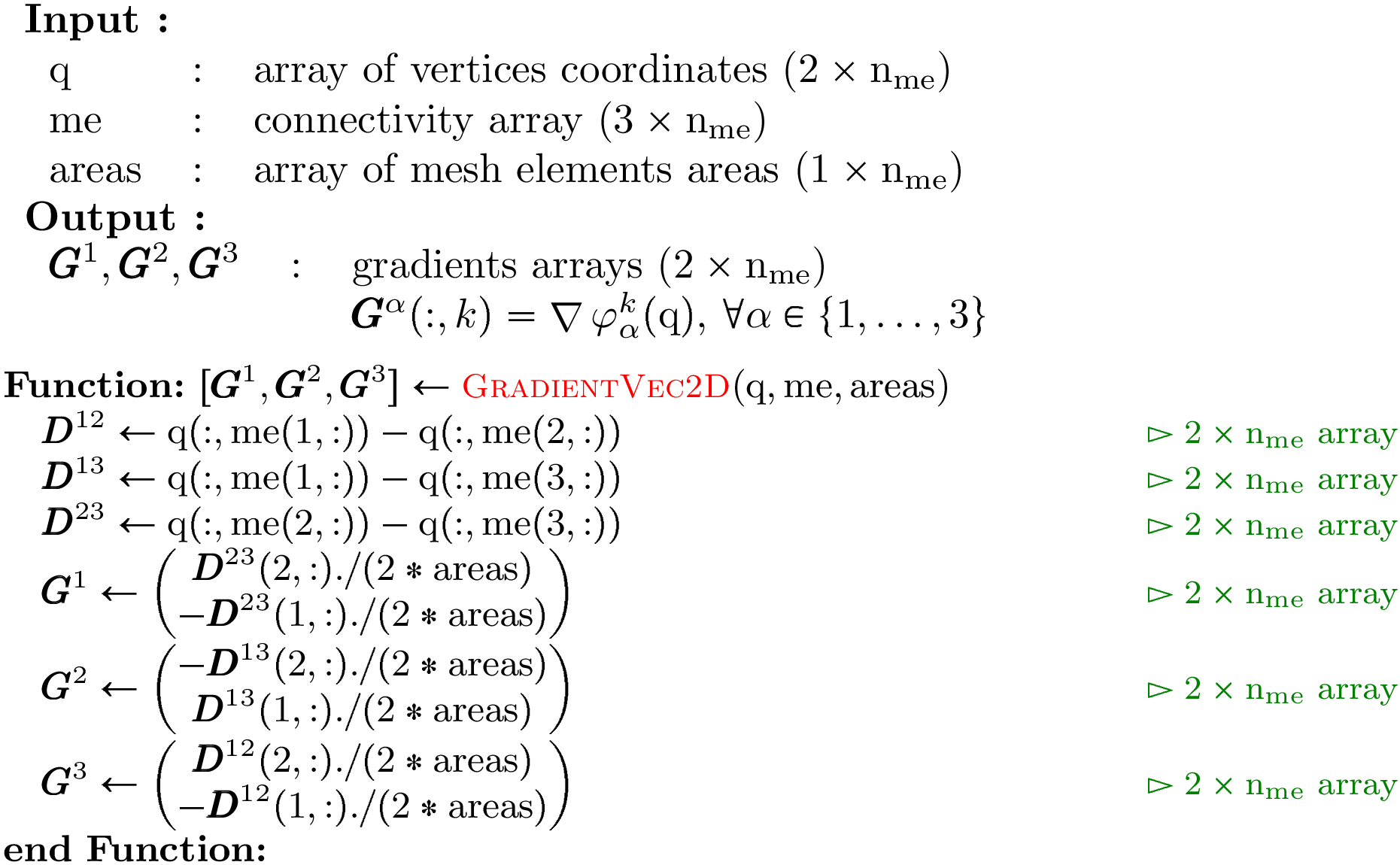
Figure 126: Vectorized algorithm for computation of basis functions gradients in 2d
Vectorized elementary matrices (used by version OptV2)
Element Mass Matrix
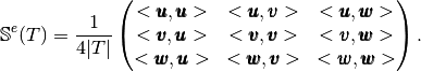
We have
Then with  definition (see Section New Optimized assembling algorithm (version OptV2)) , we obtain
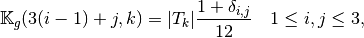
We represent in figure 135 the corresponding row-wise operations.
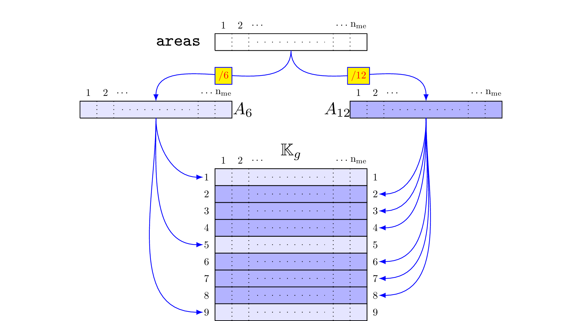
Figure 127: Build of  associated to 2d Mass matrix in
So the vectorized algorithm for computation is simple and given in Algorithm 136.
Algorithm 136
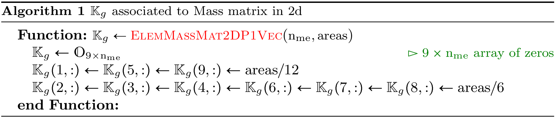
Figure 128: Vectorized algorithm for associated to 2d Mass matrix
Note
- pyOptFEM.FEM2D.elemMatrixVec.ElemMassMat2DP1Vec(areas)[source]
Compute all the elementaries Mass matrices,
 for
for 
Parameters: areas ( numpy array of floats) – areas of all the mesh elements.Returns: a one dimensional numpy array of size 
Element Stiffness Matrix
We have 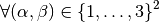
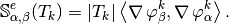
Using vectorized algorithm function  given in Algorithm 134, we obtain
the vectorized algorithm 137 for computation of the Stiffness matrix in 2d.
given in Algorithm 134, we obtain
the vectorized algorithm 137 for computation of the Stiffness matrix in 2d.
Algorithm 137
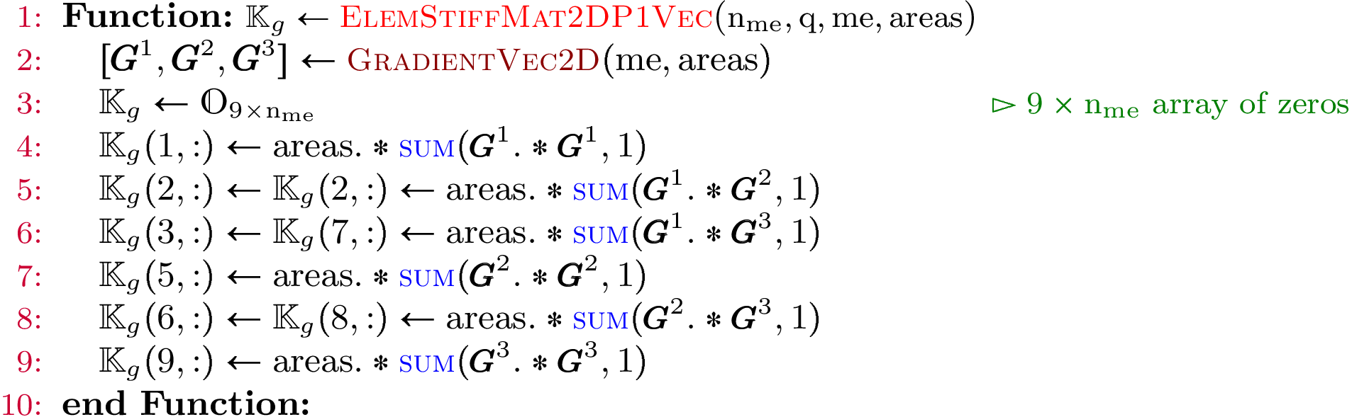
Figure 129: Vectorized algorithm for associated to 2d Stiffness matrix
Note
- pyOptFEM.FEM2D.elemMatrixVec.ElemStiffMat2DP1Vec(nme, q, me, areas)[source]
Compute all the elementaries Stiff matrices,
 for
for Parameters: - nme (int) – number of mesh elements,
- q (
 numpy array of floats) – mesh vertices,
 - me (
 numpy array of integers) – mesh connectivity,
 - areas ( numpy array of floats) – areas of all the mesh elements.
Returns: a one dimensional numpy array of size
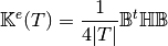
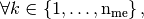
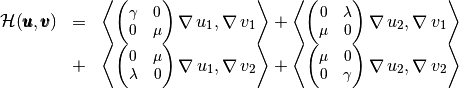
Element Stiffness Elasticity Matrix
We define on
 the local alternate basis
  by
by
where
 With notations of Presentation, we have
with,
(2)
For example, we can compute explicitely the first two terms in the first column of
 which are given by
and
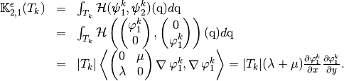
Using vectorized algorithm function
given in Algorithm 134, we obtain
the vectorized algorithm 137 for computation of the Elasticity Stiffness matrix in 2d.Algorithm 138
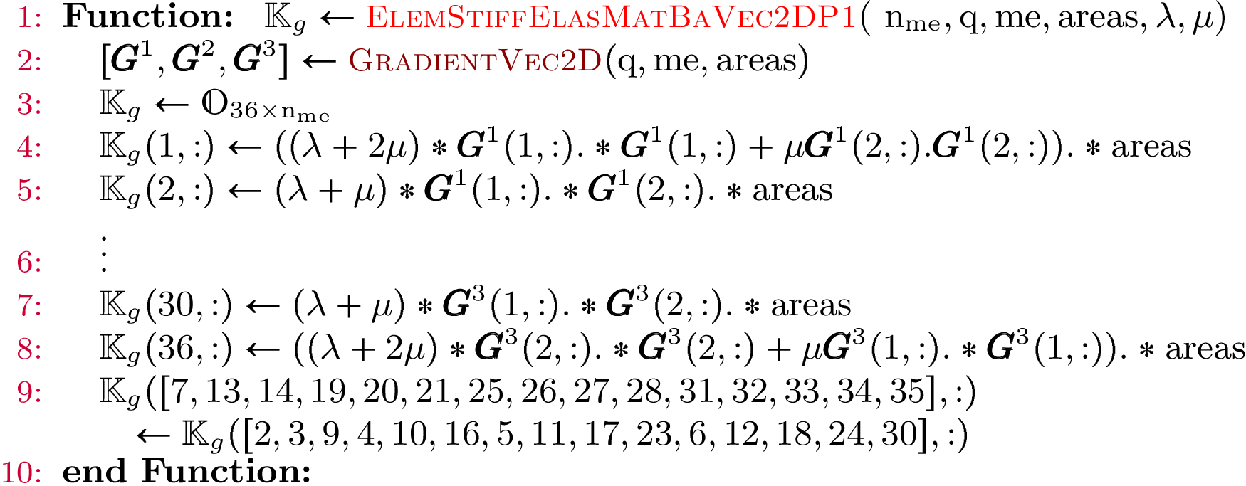
Figure 130: Vectorized algorithm for
associated to 2d Elasticity Stiffness matrixNote
- pyOptFEM.FEM2D.elemMatrixVec.ElemStiffElasMatBaVec2DP1(nme, q, me, areas, L, M)[source]
Compute all the elementaries Stiffness elasticity matrices,
 for in local alternate basis.
Parameters: - nme (int) – number of mesh elements,
- q ((2,nq) numpy array of floats) – mesh vertices,
- me ((3,nme) numpy array of integers) – mesh connectivity,
- areas ((nme,) numpy array of floats) – areas of all the mesh elements.
- L – the Lame parameter,
- L – the Lame parameter.
Returns: a (36*nme,) numpy array of floats.
We define on
the local block basis  by
by
where
For example, using formula (2), we can explicitly compute the first two terms in the first column of
which are given by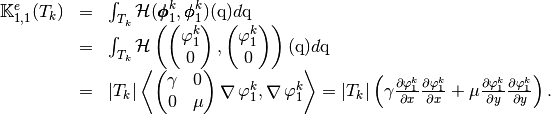
and

Using vectorized algorithm function
given in Algorithm 134, we obtain
the vectorized algorithm 139 for computation of the Elasticity Stiffness matrix in 2d.Algorithm 139
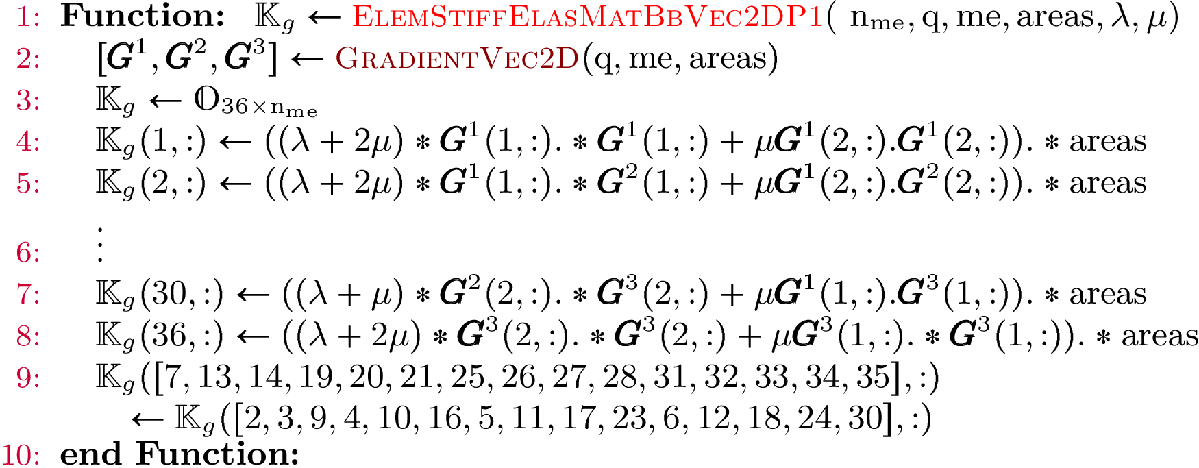
Figure 131: Vectorized algorithm for
associated to 2d Elasticity Stiffness matrixNote
- pyOptFEM.FEM2D.elemMatrixVec.ElemStiffElasMatBbVec2DP1(nme, q, me, areas, L, M)[source]
Compute all the elementaries Stiffness elasticity matrices,
for in local block basis.Parameters: - nme (int) – number of mesh elements,
- q ((2,nq) numpy array of floats) – mesh vertices,
- me ((3,nme) numpy array of integers) – mesh connectivity,
- areas ((nme,) numpy array of floats) – areas of all the mesh elements.
- L – the Lame parameter,
- L – the Lame parameter.
Returns: a (36*nme,) numpy array of floats.
Mesh
- class pyOptFEM.FEM2D.mesh.SquareMesh(N, **kwargs)[source]
Build meshes of the unit square
![[0,1]\times [0,1]](_images/math/ac8e6ab5cdf1c6a6e37ea0439ed75612939e0abb.png) . Class attributes are :
. Class attributes are :nq, total number of mesh vertices (points), also denoted
.nme, total number of mesh elements (triangles in 2d),
version, mesh structure version,
q, Numpy array of vertices coordinates, dimension (nq,2) (version 0) or (2,nq) (version 1).
q[j] (version 0) or q[:,j] (version 1) are the two coordinates of the
 -th vertex,
me, Numpy connectivity array, dimension (nme,3) (version 0) or (3,nme) (version 1).
me[k] (version 0) or me[:,k] (version 1) are the storage index of the three vertices of the
 -th triangle in the array q of vertices coordinates,
  .
.areas, Array of mesh elements areas, (nme,) Numpy array.
areas[k] is the area of
-th triangle, k in range(0,nme)
Parameters: N – points number on each sides of the square optional parameter : version=0 or version=1
>>> from pyOptFEM.FEM2D import *
>>> Th=SquareMesh(3)
>>> Th.nme,Th.nq
(18, 16)
>>> Th.q
array([[ 0.        ,  0.        ],
       [ 0.33333333,  0.        ],
       [ 0.66666667,  0.        ],
       [ 1.        ,  0.        ],
       [ 0.        ,  0.33333333],
       [ 0.33333333,  0.33333333],
       [ 0.66666667,  0.33333333],
       [ 1.        ,  0.33333333],
       [ 0.        ,  0.66666667],
       [ 0.33333333,  0.66666667],
       [ 0.66666667,  0.66666667],
       [ 1.        ,  0.66666667],
       [ 0.        ,  1.        ],
       [ 0.33333333,  1.        ],
       [ 0.66666667,  1.        ],
       [ 1.        ,  1.        ]])
>>> PlotMesh(Th)
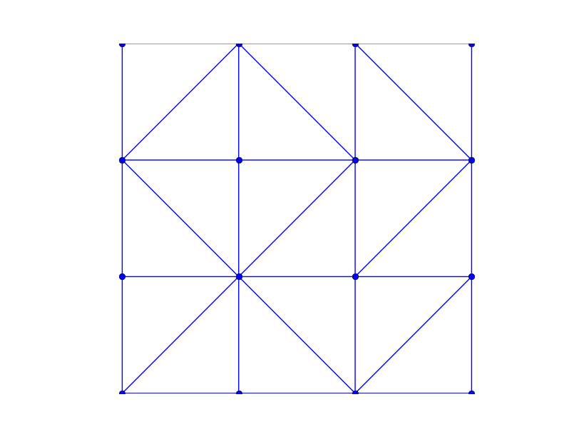
Figure 132: SquareMesh(3) visualisation
- class pyOptFEM.FEM2D.mesh.getMesh(meshfile, **kwargs)[source]
Read a FreeFEM++ mesh from file meshfile. Class attributes are :
nq, total number of mesh vertices (points), also denoted
.nme, total number of mesh elements (triangles in 2d),
version, mesh structure version,
q, Numpy array of vertices coordinates, dimension (nq,2) (version 0) or (2,nq) (version 1).
q[j] (version 0) or q[:,j] (version 1) are the two coordinates of the
-th vertex, me, Numpy connectivity array, dimension (nme,3) (version 0) or (3,nme) (version 1).
me[k] (version 0) or me[:,k] (version 1) are the storage index of the three vertices of the
-th triangle in the array q of vertices coordinates, .areas, Array of mesh elements areas, (nme,) Numpy array.
areas[k] is the area of
-th triangle, k in range(0,nme)
Parameters: N – points number on each sides of the square optional parameter : version=0 or version=1
>>> from pyOptFEM.FEM2D import *
>>> Th=getMesh('mesh/disk4-1-5.msh')
>>> PlotMesh(Th)
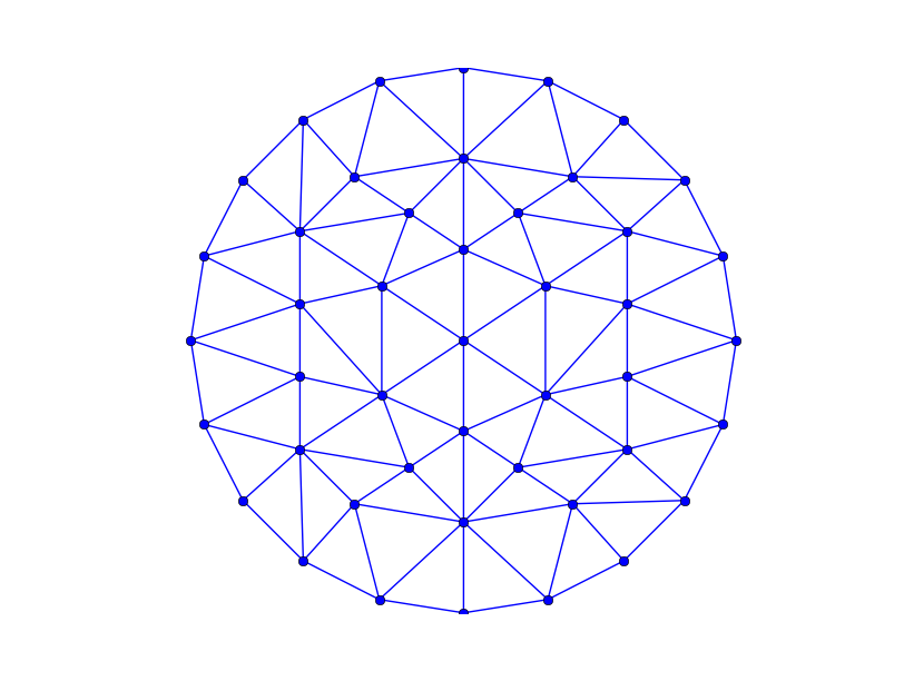
Figure 133: Visualisation of a FreeFEM++ mesh (disk unit)